Feature extraction and classification of heart sound using 1D convolutional neural networks

Feature extraction and classification of heart sound using 1D convolutional neural networks:

Abstract

We proposed a one-dimensional convolutional neural network (CNN) model, which divides heart sound signals into normal and abnormal directly independent of ECG. The deep features of heart sounds were extracted by the denoising autoencoder (DAE) algorithm as the input feature of 1D CNN. The experimental results showed that the model using deep features has stronger anti-interference ability than using mel-frequency cepstral coefficients, and the proposed 1D CNN model has higher classification accuracy precision, higher F-score, and better classification ability than backpropagation neural network (BP) model. In addition, the improved 1D CNN has a classification accuracy rate of 99.01%.

Introduction

Cardiac disorders are a high-mortality killer worldwide. According to WHO, approximately 12 million people die annually due to coronary heart disease. In the USA, 1.5 million people suffer from acute myocardial infarction, and one third of the deaths are due to coronary heart disease [1, 2]. Coronary heart disease is serious and complex. Thus, its early detection is crucial for treatment [3]. Auscultation and electrocardiogram (ECG) are two common clinical diagnostic techniques for cardiac disorders. However, ECG is ineffective in the early diagnosis of coronary heart disease. The reliable information for diagnosing coronary heart disease is provided by high-frequency murmurs from phonocardiogram (PCG) before ECG signals in patients with coronary heart disease become abnormal. Some cardiovascular system lesions first manifest as heart murmurs before causing abnormal ECG signals. Therefore, heart auscultation is the optimal choice for diagnosing these diseases. The correct classification of heart sound signals is the key technology for monitoring heart sound and providing alert for cardiovascular diseases. In addition, heart auscultation has the advantages of being noninvasive and reproducible [4]. However, raw PCG cannot intuitively determine intensity characterization and frequency of heart murmurs. In most cases, a doctor must analyze heart sounds by auscultation combined with ECG to determine patients’ heart health. Most conventional methods for automatically identifying heart sound signals rely on reference ECG signals[5–7].

The development of computer technology and digital signal processing technology has enabled recording and automatic analysis of digital heart sound signals. Spectral and time-frequency analysis methods are applied to the processing of heart sound signals, thereby constantly improving heart sound signal identification and analysis technology [8, 9]. Extracting the features of heart sound signals and performing quantitative analysis are helpful for the early screening of heart disease. Choi [10] decomposed heart sound signals to improve the accuracy of feature extraction efficiency of classification and recognition of heart sound, and Gutierrez et al. [11] used discrete wavelet transform and short-time time-frequency transform to extract heart sounds’ feature parameters; in addition, these researchers used a vectorization model to classify and recognize four kinds of common heart murmurs. Neural network pattern recognition and heart sound classification replicate doctors’ auscultation and analysis mechanism. In 1975, Karpman et al. used a standard band-pass filter and rectification detection technology to obtain the energy envelope of heart sound signals and improve the signal-to-noise ratio [12]. The diagnostic accuracy of this method was 87% in 150 patients with six types of heart disease. Gerbarg et al. [13] divided heart sounds into 0.01 s and obtained the power curve of heart sounds by calculating the average power. Existing methods use systolic and diastolic phases to determine S1 and S2 and measure parameters of mean power, peak power, time history, and peak position of systolic and diastolic phases. CotaNavin Gupta et al. [14] obtained the coefficient eigenvectors of heart sounds through Daubechies-2 wavelet decomposition and utilized them as the input of neural networks. The correct recognition rate reached 90.29% through homomorphic filtering and K-means classification method. These methods not only improve the recognition accuracy of heart sound classification but also provide a direct description of the characteristics of heart sounds. However, the application technology of heart sound signals is undeveloped. The main problem related to the development of relevant techniques is the various distinguishable pathological heart sounds and the absence of a specific extraction method for the characteristics of heart sounds. The feature extraction method has a large signal loss and does not describe the characteristics of heart sounds well. In addition, its accuracy of identification needs improvement.

In recent years, applying machine learning methods, such as support vector machine [15], learning vector quantization [16], and multivariate linear regression [17], have improved the performance of heart sound classification based on PCG signals.

In the present study, a 1D convolutional neural network (CNN) model which directly classifies heart sound signals into normal and abnormal independently of ECG is proposed. Furthermore, a denoising autoencoder (DAE) algorithm is used to extract deep features of heart sounds as the input feature to the 1D CNN rather than adopting the conventional mel-frequency cepstral coefficient (MFCC) as the input[18]. Subsequently, the 1D CNN algorithm is used to convolve the input deep feature extracted from the DAE and perform pooling operations. Finally, the processed signals are classified using a softmax classifier. We compare the deep feature extracted from the DAE with the commonly used MFCC features, thereby demonstrating the effectiveness of the deep feature of this study in the heart sound classification. Furthermore, we compare the neural network model used in this study with the backpropagation (BP) neural network, hidden Markov model (HMM), and 2D CNNs. High classification accuracy and F-score for heart sound classification are provided by the 1D CNN. The presented model is applicable to any heart sound signal collected by an electronic stethoscope and exhibits favorable robustness.

Methods

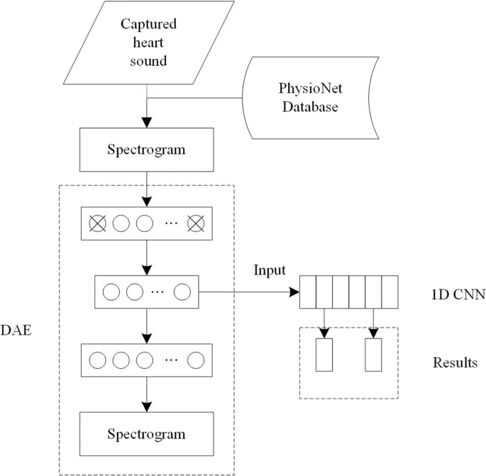
In our study, we adopted a DAE to extract the deep features of heart sound signals as the input of the 1D CNNs, and a softmax classifier was used to classify the signals. The system diagram is illustrated in Fig. 1.

Fig. 1

Overall structure of the system

Full size image

PCG data processing

Database acquisition

The datasets used in this study include two parts: part 1 was collected by our research team, and part 2 was downloaded from the PhysioNet database [19]. Part 1 consists of the heart sounds we collected in the laboratory. Each heart sound lasted from 20 s to 35 s, and all of them were collected by placing the electronic stethoscope at the strongest point of the tester’s apex, which is the fifth intercostal space on the inner side of the left clavicular midline. The participants were 45 adults, consisting of 30 males and 15 females, aged 22–38 years. Among the participants, 43 were healthy and 2 had a confirmed cardiac diagnosis. Part 2 was downloaded from the PhysioNet database, which includes 4430 recordings taken from 1072 subjects, totaling 233,512 heart sounds collected from healthy subjects and patients various conditions, such as heart valve disease and coronary artery disease. These recordings were collected using heterogeneous equipment in clinical and nonclinical settings (such as in-home visits). The length of recording varied from 5 s to 120 s. The recordings were collected from different locations on the body. A total of 2532 recordings were collected from healthy subjects, and 664 were collected from patients with confirmed cardiac diagnoses. Healthy subjects and pathological patients included children and adults.Each subject/patient possibly contributed between one and six heart sound recordings. Combining the two parts, we obtained the datasets used in this study.The dataset can be divided into two types, namely, normal and abnormal. All recordings were resampled to 2000 Hz, and each recording contained only one PCG lead. Figure 2 depicts a schematic of the hardware composition of the heart sound signal detection system.

Fig. 2

Schematic of the hardware composition of the heart sound signal detection system

Full size image

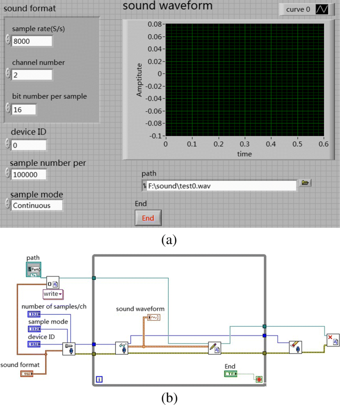
To acquire the heart sound of the subject, the heart sound acquisition tool is Yuwell electronic stethoscope, as shown in Fig. 3. The heart sound were captured with the Labview software (as shown in Fig. 4a) via the sound card of the computer with a sampling rate of 2 kHz and 16 bits. A Core i5 3.0 GHz Intel (R) personal computer with 8.00 GB ram running Microsoft Windows 7 operating system is used.

Fig. 3

Yuwell electronic stethoscope

Full size image

Fig. 4

The block diagram of heart sound signal acquisition and corresponding block diagram. a Block diagram of heart sound signal acquisition. b Corresponding block diagram

Full size image

Taking into account the performance of the sound card, the sampling frequency of the system is set to 2000 Hz, the number of samples is set to 16 bits, and the sampling mode is single channel, so that the sampling waveform is stable and the interference is small. The waveforms can be observed through the functions provided by the Labview waveform monitor when heartbeat acquisition is paused and terminated. The collected data (the part 1 mentioned in “Database acquisition” section) is also saved in the.wav format and performs the same operations as the data in the PhysioNet Database. Figure 4 shows the block diagram of heart sound signal acquisition.

Sample expansion

The structure of the CNNs was simplified as a basic structure of a convolution layer, a sampling layer, and a full network layer to compare the influence of two CNNs on heart sounds. We trained the 2D CNN models with the same number of layers. The convolution layer had 20 feature maps, and the transfer function was sigmoid(). The pooling layer used max-pooling, and the stride was 2. The softmax classifier was used to output the posterior probability of each class. The extraction of an autoencoder feature was used to verify the description of the sound signal well. The heart sound window was pretreated. The extracted MFCC coefficient of the traditional 1D CNNs was used as the input of the networks, and the deep features are compared.

The minimum duration of heart sound acquisition was 5 s. In this study, we divided the signals into pieces of 5 s, and the most common smoothing windows were selected. First, we trained the classifier for each segment extracted from the records to classify normal and abnormal heart sound signals, rather than extract from the entire record [20]. The classifier not only extended the sample size of the entire dataset but also reduced the overfitting in network training by expanding the sample size of the dataset and then the merging the lengths of all the samples.

Training and test data

We obtained 13,015 samples after expanding the data. Deep learning requires numerous samples to train for improved generalization. In comparison with the amount of image data processed by CNNs [21, 22], the datasets used in our experiment were minimal. To obtain as much effective information as possible from limited data, we adopted K-fold cross-validation to process the data and obtain the training and the test sets. The training set contained 9761 samples, and the test set contained 3245 samples.

Feature extraction based on the dAE

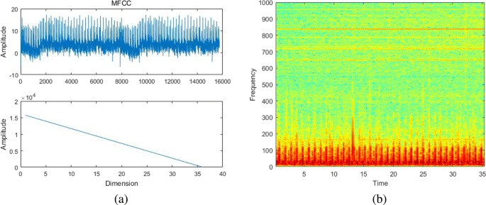
Feature extraction aims to extract the identifiable components of the original signal. The MFCC is widely used in automatic speech and speaker recognition[23, 24]. It was proposed by Davis and Mermelstein in the 1980s and had constantly played an important role in speech recognition. The mel-frequency analysis is based on human auditory perception. The experimental results show that the human ear acts like a filter bank, thereby focusing only on certain frequency components. That is, it only transmits signals of certain frequencies and directly ignores undesired signals. Thus, information loss remains large when these feature parameters are applied to the time and the frequency domains. In the MFCC algorithm [25], the signal is first framed and the Hamming window is used to reshape the audio signal into small windows. Using the fast Fourier transform, the spectrum is calculated for each frame, and each spectrum is weighted using a filter bank. Finally, the MFCC vector is calculated using logarithmic and discrete cosine transforms. During feature extraction, we re-sampled each signal frequency to 16 kHz and set the number of filter to 40 and the filter order to 24. Each sample had a time frame of 25 ms, and stride was 10 ms (15 ms overlap). The MFCC of the heart sound is depicted in Fig. 5a. No intuitive signal frequency characteristic was observed in the time domain. Moreover, the heart sound exhibited a diverse acquisition environment and the signal itself was relatively weak in comparison with the noise. Therefore, the MFCC as a speech feature parameter cannot fully represent the characteristic parameters of heart sounds. In this study, we adopted the DAE network to obtain the feature parameters of heart sound signals. Figure 5b shows a spectrogram of a heart sound, which is a visual representation of the spectrum of frequencies of a signal while it varies with time. A time-varying spectrogram is typically obtained by processing the received time domain signal, thereby enabling us to observe the formants and the attributes of the phonemes in the signal intuitively. In 2011, Deng et al. [26] demonstrated that when a speech feature is encoded using a autoencoder using unsupervised learning, speech coding can be extracted directly from the spectrogram data of the original speech signal for feature recognition. As mentioned previously, we used the DAE network which inputs a spectrogram to extract the feature of the heart sound signal.

Fig. 5

The mfcc and spectrogram of the heart sound. a The mfcc of the heart sound. b The spectrogram of the heart sound

Full size image

The main principle of the autoencoder is that the original input (set as x) obtains y after weighting (W, b) and mapping (sigmoid function or tanh function), and then maps back to y in inverse weighting as z. Perfect reconstruction is performed by iteratively training (W, b) to minimize the error of the function, that is, to ensure that z is as close to x as possible. The process of mapping x to y can be expressed as follows:

y=sigmoid(Wx+b),$$y=sigmoid(Wx+b),$$

(1)

where sigmoid() is transfer function. This process is called the encoder. y is mapped back to the reconstruction vector z, which is called process decoder.

z=sigmoid(W′y+b′),$$z=sigmoid(W^{\prime }y+b^{\prime }),$$

(2)

where W is the weight, and b is the bias.The weight matrix W′ may be left as a transpose of the encoder weight matrix W′=WT.

The entire process can be considered a reconstruction process. The loss function is expressed as follows:

• Squared difference:
  L(xz)=∥x−z∥2$$L(xz)=\Vert x-z{\Vert }^2$$

  (3)
• Cross entropy:
  LH(xz)=−∑k=1s[xklogzk+(1−xk)log(1−zk)]$$L_H(xz)=-\sum _{k=1}^s[x_k\text{log}{z}_k+(1-x_k)\text{log}(1-z_k)]$$

  (4)

In this study, we adopted a DAE algorithm for feature extraction of original heart sound data from each person in the database. The DAE is an extension of the autoencoder and was introduced in the deep network Vincent 08 [27]. To prevent overfitting, noise is added to the input data (the input layer of the network), thereby making the learned encoder robust and enhancing the generalization capability of the model. The raw data in the DAE are reconstructed by training the samples with noise. One way to add noise is to zero some elements of the input signal randomly using a binomial distribution with parameters n and p (in this study, n and p correspond to the number of pixels of the spectrogram and 40%). The DAE is trained to reconstruct a clean “repaired” input from a corrupted version of which the elements is randomly set to 0 [28]. With this missing data, x′ to calculate y, z is calculated, and error iterations are conducted with z and original x. Thus, the corrupted data are learned by the network. The advantage of this method is that, in comparison with the non-destructive data training, the weight noise trained by the damage data is relatively small, and the damage data reduce the difference between the training and the test data. The robustness is improved, as displayed in Fig. 6.

Fig. 6

DAE used in this study

Full size image

1D cNNs for the proposed system

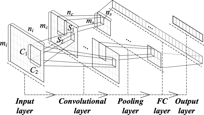
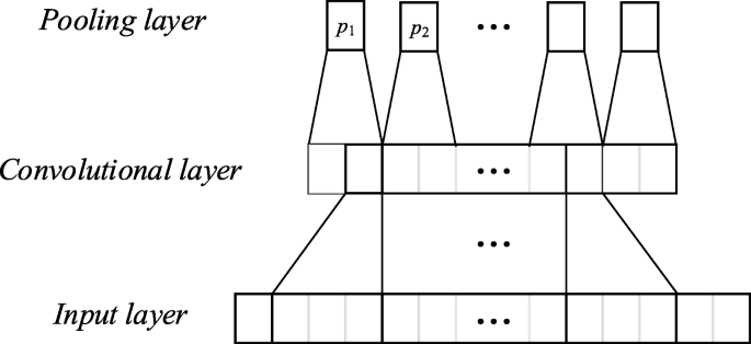
In 2012, Abdel-Hamid [29] introduced CNNs into speech recognition and preliminarily identified the basic structure of the networks, in which the convolution and pooling layers alternately appeared. The scale of the convolution kernel is large, and the number of CNN layers is minimal. The CNNs used in the speech recognition task is a 2D model, although language is a typical 1D signal. A typical CNN structure is presented in Fig. 7. The convolution kernel, feature map, and other network structures are 2D. At present, when processing a 1D signal with CNNs, the 1D signal is usually mapped to a 2D space (for example, a 1D speech signal can be converted into 2D feature maps [30], static feature maps [31], or frequency-time feature [32]). Then, these 2D features are input into the conventional 2D CNNs for further processing. To observe local characteristics and capability construction of the long band signal, the traditional approach is to divide the speech into frames, extract the feature parameters, and arrange them by column to constitute long-term features. However, the meanings of the two dimensions are different, that is, one is the time domain features and the other is frequency characteristics. The 2D CNNs cannot adapt well to the 1D characteristics of speech because two dimensions have completely different physical meanings.

Fig. 7

Typical CNN structure

Full size image

The characteristics of the 1D audio signal, that is, the 1D vector as the input to the CNNs, were used in this study. Thus, the convolution kernel and characteristic map inside the networks were also 1D, and the values of mi,Ci,mc,Si, and ms in the graph were all 1. Yij represents the value of location y on layer i in feature graph j and can be convoluted through the 1D vector of the upper layer and 1D convolution kernel, as follows:

Vyij=tanh(bij+∑m∑l=0liωlijmVy+l(i−1)m)$$V_{ij}^y=\tanh (b_{ij}+\sum _m\sum _{l=0}^{l_i}{\omega }_{ijm}^l{V}_{(i-1)m}^{y+l})$$

(5)

where tanh() is a transfer function, bij is the bias of the feature map, m is the ordinal number of the set of characteristic graphs connected to the characteristic graph in the (i−1) level, and represents the value of position l in the convolution kernel of the characteristic graph connected to serial number m, and li represents the length of the convolution kernel in layer i.

Figure 8 exhibits the structure of the convolution and sampling layers when the 1D CNNs were used for modeling heart sound recognition. In the CNN input, we only used the features of the 5 s signal extracted from the automatic encoder to form the first dimension of the CNNs. The physical meaning of the convolution layer is to extract certain useful information from a convolution, which is similar to a filter. It directly determines the overall performance of the networks through the shape and size of the convolution kernel. The correlation information of the input signal will be lost in the extracted feature when the convolution kernel is small. A 1D convolution kernel that typically corresponds to the long signal frames is used to extract additional features. The sampling layer (pooling) will sample the feature graph that is extracted from the coiling layer. In this study, the maximum value of the pool area is used as the point after pooling. All features were 1D vectors and could be connected directly one by one. We applied the full connection layer to generate an output that is equal to the number of classes to generate the final output.

Fig. 8

Sample diagram of coiling and maximum sampling layers in CNNs

Full size image

The output layer has a loss function similar to the classification cross entropy, which is used to calculate the prediction error. After forward propagation, the BP is conducted to update the weights and deviations. Thus, the error and loss are reduced.

Experiments and results

In this section, we perform three comparative experiments. The first one compares different convolution kernel shapes, the second one compares various features, and the third one compares of the different numbers of the network layer. In the statistical analysis of binary classification, the F- score indicates a test’s accuracy [33].The F-score is the harmonic mean of the precision and recall, where an F-score reaches its optimal value at 1 and worst at 0. In this study, we use the F-score and recognition accuracy rate to quantify the performance of the method, F-score can be calculated using the following equation.

F−score=2×TPTP+FP×TPTP+FNTPTP+FP+TPTP+FN$$F-\mathrm{s}\mathrm{c}\mathrm{o}\mathrm{r}\mathrm{e}=2\times \frac{\frac{TP}{TP+FP}\times \frac{TP}{TP+FN}}{\frac{TP}{TP+FP}+\frac{TP}{TP+FN}}$$

(6)

Accuracy=TP+TNTP+TN+FP+FN$$A\mathrm{c}\mathrm{c}\mathrm{u}\mathrm{r}\mathrm{a}\mathrm{c}\mathrm{y}=\frac{TP+TN}{TP+TN+FP+FN}$$

(7)

where TP denotes true positive, FP signifies false positive, FN indicates false negative, and TN implies true negative.

Comparison of different convolution kernel shapes

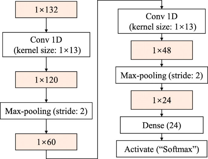
A vector of 1×132 dimension is utilized as the 1D CNN feature input. We train 2D CNN models with the same construction as the 1D CNNs we proposed. Each model has a convolution layer with 20 feature maps, and the transfer function is sigmoid. The pooling layer uses max-pooling, and the stride is 2. The softmax classifier is used to make the output result a posterior probability of each class. Taking the five-layer 1D CNN with a convolution kernel size of 1×13 as an example, the network structure is depicted in Fig. 9.

Fig. 9

Network structure of the proposed 1D CNNs

Full size image

We extend the 2D convolution kernel to the corresponding 1D convolution kernel based on column expansion. To compare the effects of different convolution kernel shapes on the performance of two CNNs, maintain the convolution kernels at the same size in both networks, but change the shape to the corresponding 1D and 2D forms. In Table 1, 1×26 represents the length of convolution kernel 26, and the corresponding 2D convolution kernel is 2×13. The experimental results displayed in Table 1 indicate that, under the same convolution kernel size, when the convolution kernel is increased from 1D to 2D, the recognition accuracy is reduced, and the maximum amplitude is approximately 3% (when the convolution kernel size is 39). When changing the convolution kernel shape, the recognition accuracy is constantly kept at approximately 1∼3% higher in the 1D CNNs than in the 2D CNNs.

Table 1 Comparison results of different convolution kernels

Full size table

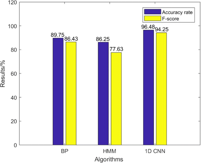
Figure 10 shows that, in comparison with other classification methods, such as BP neural network, the recognition accuracy is 89.75%, and the final recognition rate of the method used in this paper is increased by nearly 7%. The BP neural network uses the same number of weight parameters as the 1D CNNs. The number of states in the HMM is 6, and the probability distribution of the observed signal is approximated by three Gaussian distributions.

Fig. 10

Comparison of recognition results of different algorithms

Full size image

Comparison of different features

We have conducted several sets of contrast experiments to verify that the feature extraction method used in this study is superior to the traditional MFCC features. The experimental results are summarized in Table 2.

Table 2 Comparison results of different features in 1D CNNs

Full size table

Table 2 shows that the deep features extracted in this study exhibit favorable recognition rates, thereby indicating that the extracted features can filter out noise and interference sound well and adapt to the characteristics of the networks favorably.

Comparison of different numbers of network layer

To obtain enhanced results, we use the proposed 1D CNNs and then add a layer of neural networks to form a two-layer CNNs. In the CNN structure, the convolution and pool layers alternately appear. The convolution and pool layers are added. Finally, the layers are fully connected to obtain the output. We compare the performance of the network under different layers. We find that the performance of the network remains the same when the number of layers exceeds 5. The experimental results are presented in Table 3. The results indicate that the increase in the convolution layer has improved the recognition accuracy of the signal for the samples in this study.

Table 3 Results of the different numbers of convolution layers in 1D CNNs

Full size table

Discussion

The experimental results denote that the deep features used in the proposed system retain additional details of heart sound signals, thus improving the classification performance.The results in Table 1 show that the classification accuracy is higher in the 1D CNN than in the 2D CNN for the heart sound signals used in this study when the convolution kernel is less than 52 because a large convolution kernel can lead to computational complexity and is increasingly time- consuming. By comparing the traditional speech feature MFCC and the deep feature extracted in this study, the latter is nearly 7% higher than that of the former in the correct rate of the final classification recognition. Therefore, the deep feature extracted in this study is more suitable for representing heart sound signals than that of the MFCC. Moreover, the recognition accuracy is high when the number of layers is also high. However, with the increase in the number of layers, the amount of calculation slightly increases, and the duration of classification recognition is prolonged.

In comparison with the traditional input for any length of heart sound, the extraction of the deep features does not require preprocessing. Thus, the heart sound can be directly inputted into the networks for classification. In this study, applying the 1D CNN model rather than 2D CNNs significantly improves the capability of the entire network model to recognize heart sound signals. The proposed method can achieve reliable recognition performance based on acoustic characteristics without using reference ECG.

The model proposed in this study can be used for routine testing in daily life or clinical setting for the general population. If an abnormality occurs, then visiting the hospital for further examination is necessary. Limited by the number of the samples we collected, this method can only classify normal/abnormal heart sounds at present. Thus, it has not been applied in clinical practice but can be used for early warning of heart disease. In the future,we can further improve the algorithms and sample collection for application in clinical practice.

Conclusion

In this study, we propose a method based on DAE and depth 1D CNNs to characterize and classify the PCG. Through the experimental analysis, the following conclusions can be obtained:

• The classification performance of the feature parameters extracted by autoencoder is better than those extracted by the extensively used MFCC.
• 1D CNNs improve the classification accuracy by 1%. These algorithms are improved on the basis of 2D CNNs.
• The system proposed in this study can classify heart sounds based on the acoustic features independently of the ECG and does not need to preprocess the signal,which has certain universality.

In summary, the model proposed in this study can effectively improve the classification accuracy of heart sounds. This result is crucial for the further realization of automatic diagnosis of heart disease.

Availability of data and materials

The part 1 of databases supporting the conclusions of this article are not available because it refers to subjects’ personal privacy. We will protect the privacy right of subjects to the maximum extent possible.

The part 2 of databases supporting the conclusions of this article are available in the [PhysioNet Database] repository [unique persistent identifier and hyperlink to datasets in http://www.physionet.org:8080/physiobank/database/].

Abbreviations

CNNs:

Convolutional neural networks

DAE:

Denoising autoencoder

DAE:

Denoising autoencoders

ECG:

Electrocardiogram

LVQ:

Learning vector quantization

MFCC:

Mel-frequency cepstral coefficient

MLR:

Multivariate linear regression

PCG:

Phonocardiogram

SVR:

Support vector machine

References

1. 1
   M. Hossain, Global, regional, and national ageŰsex specific all-cause and cause-specific mortality for 240 causes of death, 1990-2013: a systematic analysis for the Global Burden of Disease Study 2013[J]. Lancet. 385(9963), 117–171 (2014).
   • Google Scholar
2. 2
   Y. Hui, J. M. Garibaldi, A hybrid model for automatic identification of risk factors for heart disease. J. Biomed. Inform.58(Suppl), S171–S182 (2015).
   • Google Scholar
3. 3
   W. Koenig, Epidemiology of coronary heart disease. Z. Kardiol.87(Suppl 2), 3 (1998).
   • Article
   • Google Scholar
4. 4
   R. M. Rangayyan, R. J. Lehner, Phonocardiogram signal analysis: a review. Crit. Rev. Biomed. Eng.15(3), 211–236 (1987).
   • Google Scholar
5. 5
   P. Tadejko, W. Rakowski, in International Conference on Computer Information Systems & Industrial Management Applications. Mathematical morphology based ecg feature extraction for the purpose of heartbeat classification (IEEE, 2007). https://doi.org/10.1109/cisim.2007.47.
6. 6
   L. Jia, D. Song, L. Tao, et al., Heart sounds classification with a fuzzy neural network method with structure learning[C]. International Symposium on Neural Networks (Springer, Berlin, Heidelberg, 2012).
   • Google Scholar
7. 7
   E. J. D. S. Luz, W. R. Schwartz, G. Cámara-Chávez, D. Menotti, ECG-based heartbeat classification for arrhythmia detection: A survey. Comput. Methods Programs Biomed.127(C), 144–164 (2016).
   • Article
   • Google Scholar
8. 8
   D. W Sapire, Understanding and diagnosing pediatric heart disease[M]. Appleton & Lange (1991).
9. 9
   X. Zhang, L. G. Durand, L. Senhadji, H. C. Lee, J. L. Coatrieux, Analysis-synthesis of the phonocardiogram based on the matching pursuit method. IEEE Trans. Bio-med. Eng.45(8), 962–71 (1998).
   • Article
   • Google Scholar
10. 10
    S. Choi, Detection of valvular heart disorders using wavelet packet decomposition and support vector machine. Expert Syst. Appl.35(4), 1679–1687 (2008).
    • Article
    • Google Scholar
11. 11
    F. Rios-Gutierrez, R. Alba-Flores, K. Ejaz, G. Nordehn, N. Andrisevic, S. Burns, in The 2006 IEEE International Joint Conference on Neural Network Proceedings. Classification of four types of common murmurs using wavelets and a learning vector quantization network (IEEE, 2006). https://doi.org/10.1109/ijcnn.2006.1716385.
12. 12
    L. Karpman, J. Cage, C. Hill, A. D. Forbes, V. Karpman, K. Cohn, Sound envelope averaging and the differential diagnosis of systolic murmurs. Am. Heart J.90(5), 600–606 (1975).
    • Article
    • Google Scholar
13. 13
    D. S. Gerbarg, Fw Holcomb Jr, J. J. Hofler, C. E. Bading, G. L. Schultz, R. E. Sears, Analysis of phonocardiogram by a digital computer. Circ. Res.11:, 569 (1962).
    • Google Scholar
14. 14
    C. N. Gupta, R. Palaniappan, S. Swaminathan, S. M. Krishnan, Neural network classification of homomorphic segmented heart sounds. Appl. Soft Comput.7(1), 286–297 (2007).
    • Article
    • Google Scholar
15. 15
    S. Ghumbre, C. Patil, A. Ghatol, Heart disease diagnosis using support vector machine[C]. International conference on computer science and information technology (ICCSIT’). Pattaya (2011).
16. 16
    A. H. Chen, S. Y. Huang, P. S. Hong, C. H. Cheng, Hdps: Heart disease prediction system. Comput. Cardiol.557–560: (2011).
17. 17
    V. Giancarlo, C. A. Lage, V. Gianluca, F. Elia, Multivariate linear regression of high-dimensional fmri data with multiple target variables. Hum. Brain Mapp.35(5), 2163–2177 (2014).
    • Article
    • Google Scholar
18. 18
    L. R. Rabiner, B. H. Juang, Fundamentals of speech recognition[M] (Tsinghua University Press, 1999).
19. 19
    A. L. Goldberger, L. A. Amaral, L. Glass, J. M. Hausdorff, P. C. Ivanov, R. G. Mark, J. E. Mietus, G. B. Moody, C. K. Peng, H. E. Stanley, Physiobank, physiotoolkit, and physionet: components of a new research resource for complex physiologic signals. Circulation. 101(23), E215 (2000).
    • Article
    • Google Scholar
20. 20
    T. Nilanon, J. Yao, J. Hao, S. Purushotham, Y. Liu, Normal / abnormal heart sound recordings classification using convolutional neural network. Comput. Cardiol. Conf. (2017). https://doi.org/10.22489/cinc.2016.169-535.
21. 21
    T. Y. Lin, M. Maire, S. Belongie, J. Hays, P. Perona, D. Ramanan, P. Dollár, C. L. Zitnick, in Computer Vision ? ECCV 2014. Microsoft coco: Common objects in context, (2014), pp. 740–755. https://doi.org/10.1007/978-3-319-10602-1_48.
    • Google Scholar
22. 22
    Y. Li, M. Y. Liu, X. Li, M. H. Yang, J. Kautz, in Computer Vision ? ECCV 2018. A closed-form solution to photorealistic image stylization, (2018), pp. 468–483. https://doi.org/10.1007/978-3-030-01219-9_28.
    • Google Scholar
23. 23
    S. Jothilakshmi, V. Ramalingam, S. Palanivel, Unsupervised speaker segmentation with residual phase and MFCC features. Expert Syst. Appl.36(6), 9799–9804 (2009).
    • Article
    • Google Scholar
24. 24
    Rajsekhar A.G., Real time speaker recognition using MFCC and VQ[J]. Department of Electronics & Communication Engineering National Institute of Technology Rourkela (2008).
25. 25
    A. P Nair, S Krishnan, Z Saquib, MFCC based noise reduction in asr using kalman filtering. Adv. Sig. Process (2016).
26. 26
    L. Deng, M. L. Seltzer, D. Yu, et al., Binary coding of speech spectrograms using a deep auto-encoder[C]. Eleventh Annual Conference of the International Speech Communication Association (2010).
27. 27
    P Vincent, H Larochelle, Y Bengio, P. A Manzagol, in Proceedings of the 25th international conference on Machine learning - ICML ’08. Extracting and composing robust features with denoising autoencoders (ACM Press, 2008). https://doi.org/10.1145/1390156.1390294.
28. 28
    P Vincent, H Larochelle, I Lajoie, Y Bengio, P. A Manzagol, Stacked denoising autoencoders: Learning useful representations in a deep network with a local denoising criterion. J. Mach. Learn. Res. 11(12), 3371–3408 (2010).
    • MathSciNet
    • MATH
    • Google Scholar
29. 29
    O Abdel-Hamid, A. R Mohamed, H Jiang, G Penn, in 2012 IEEE International Conference on Acoustics, Speech and Signal Processing (ICASSP). Applying convolutional neural networks concepts to hybrid NN-HMM model for speech recognition (IEEE, 2012). https://doi.org/10.1109/icassp.2012.6288864.
30. 30
    O Abdel-Hamid, A. R Mohamed, H Jiang, L Deng, G Penn, D Yu, Convolutional neural networks for speech recognition. IEEE/ACM Trans. Audio Speech Lang. Process. 22(10), 1533–1545 (2014).
    • Article
    • Google Scholar
31. 31
    Y Qian, P. C Woodland, Very deep convolutional neural networks for robust speech recognition. IEEE/ACM Trans. Audio Speech Lang. Process. 24(12), 2263–2276 (2016).
    • Article
    • Google Scholar
32. 32
    V Mitra, G Sivaraman, H Nam, C Espy-Wilson, E Saltzman, M Tiede, Hybrid convolutional neural networks for articulatory and acoustic information based speech recognition. Speech Commun. 89(C), 103–112 (2017).
    • Article
    • Google Scholar
33. 33
    M. Sokolova, N. Japkowicz, S. Szpakowicz, Beyond accuracy, F-score and ROC: a family of discriminant measures for performance evaluation[C]. Australasian joint conference on artificial intelligence (Springer, Berlin, Heidelberg, 2006).
    • Google Scholar

Download references

Acknowledgements

This work was supported by The National Natural Science Fund of China (grant numbers 61705010, 61301190).

Author information

Affiliations

1. Beijing Key Laboratory for Precision Optoelectronic Measurement Instrument and Technology, School of Optics and Photonics, Beijing Institute of Technology, Beijing, 100081, China

   • Fen Li
   • , Ming Liu
   • , Yuejin Zhao
   • , Lingqin Kong
   • , Liquan Dong
   • , Xiaohua Liu
   •  & Mei Hui

Contributions

Authors’ contributions

FL, ML, YZ, LK, LD, XL, and MH conceptualized and designed the study. FL acquired and analyzed the data,drafted the text, and prepared the figures. All authors read and approved the final version of the manuscript to be published.

Authors’ information

Li F. received her B.S. degrees from the School of Manufacturing Science and Engineering, Sichuan University, Sihuan, China; she is currently a PH.D. student in School of Optics and Photonics, Beijing Institute of Technology. Her research interest covers Medical Signal Processing, intelligent image processing, object detection, and deep learning.

Liu M. received his B.S. degrees from the School of Information, Shandong University, Shandong, China, and M.S. degrees and Ph.D degrees from the School of Optics and Photonics at Beijing Institute of Technology in 2006 and 2009 respectively. He is currently an associate professor in School of Optics and Photonics, Beijing Institute of Technology. His research interest covers intelligent image processing, object detection, machine vision optics.

Zhao Y.J. is a professor of Beijing Institute of Technology, School of Optics and Photonics. He received his PhD degree in optical engineering, Beijing Institute of Technology in June 1990. Currently, he is a disciplinary responsibility to the team leader of “Instrument Science and Technology” in Beijing Institute of Technology. He has been engaged in teaching and research work in the field of optoelectronic instruments. His current research interests include terahertz imaging technology based on MEMS-infrared imaging technology, space optical technology, and intelligent photoelectric instrument development. He is the deputy director of the Standing Committee of Optical Society of China, vice chairman of China Instrument Society of Optical and Electrical Machinery and Systems Integration Technology branch.

Kong L.Q. received the B.S. and M.S. degrees in physical electronics from the Taiyuan University of Technology, Taiyuan, China, in 2006 and 2009, respectively, and the Ph.D. degree in instrument science and technology from the Beijing Institute of Technology, Beijing, China, in 2014. She is currently a Lecturer and the Master’s Tutor with the Beijing Institute of Technology. Her current research interests include video processing for vital signs, optical system design, and high-speed aero optic effects.

Dong L.Q. received his B.S degree and Ph.D degree from the School of Optics and Photonics at Beijing Institute of Technology, Beijing, China, in 2000 and 2007 respectively. He is currently an associate professor and the vice-president in the School of Optoelectronic. His research interests include photoelectric instrument and detection technology, video and image processing, and infrared night-vision technology.

Liu X.H. is an associate professor with the Advanced Photoelectric Instrument Laboratory in Beijing Institute of Technology. He received his BS degree from the Department of Physics, Peking University, in 1983 and his MS degree from the Department of Optical Engineering, Beijing Institute of Technology, in 1988. His current research interests include the terahertz technology, infrared imaging, and advanced imaging systems.

Hui M. received her PhD degree from Xi’an Institute of Optics and Precision Mechanics of Chinese Academy of Science in 2001. She is currently an associate professor in the School of Optoelectronics, Beijing Institute of Technology. Her current research interests include phase-shifting interferometry, segmented mirror co-phasing testing, infrared MEMS system imaging, and mechanical design.

Corresponding author

Correspondence to Ming Liu.

Ethics declarations

Ethics approval and consent to participate

In this study, the rights and interests of the subjects are fully protected and there is no potential risk to the subjects. The ethical review report is attached.

Additional information

Publisher’s Note

Springer Nature remains neutral with regard to jurisdictional claims in published maps and institutional affiliations.

Rights and permissions

Open Access This article is distributed under the terms of the Creative Commons Attribution 4.0 International License(http://creativecommons.org/licenses/by/4.0/), which permits unrestricted use, distribution, and reproduction in any medium, provided you give appropriate credit to the original author(s) and the source, provide a link to the Creative Commons license, and indicate if changes were made.

Reprints and Permissions